
通过Sub-Pixel实现图像超分辨率
日期: 2021.01
摘要: 本示例教程使用U-Net实现图像分割。
在计算机视觉中,图像超分辨率(Image Super Resolution)是指由一幅低分辨率图像或图像序列恢复出高分辨率图像。图像超分辨率技术分为超分辨率复原和超分辨率重建。
本示例简要介绍如何通过飞桨开源框架,实现图像超分辨率。包括数据集的定义、模型的搭建与训练。
参考论文:《Real-Time Single Image and Video Super-Resolution Using an Efficient Sub-Pixel Convolutional Neural Network》
论文链接:https://arxiv.org/abs/1609.05158
二、环境设置
本案例使用BSR_bsds500数据集,下载链接:
!wget --no-check-certificate --no-cookies --header "Cookie: oraclelicense=accept-securebackup-cookie" http://www.eecs.berkeley.edu/Research/Projects/CS/vision/grouping/BSR/BSR_bsds500.tgz!tar -zxvf BSR_bsds500.tgz
--2021-01-29 00:11:52-- http://www.eecs.berkeley.edu/Research/Projects/CS/vision/grouping/BSR/BSR_bsds500.tgzResolving www.eecs.berkeley.edu (www.eecs.berkeley.edu)... 23.185.0.1, 2620:12a:8001::1, 2620:12a:8000::1Connecting to www.eecs.berkeley.edu (www.eecs.berkeley.edu)|23.185.0.1|:80... connected.HTTP request sent, awaiting response... 301 Moved PermanentlyLocation: https://www.eecs.berkeley.edu/Research/Projects/CS/vision/grouping/BSR/BSR_bsds500.tgz [following]--2021-01-29 00:11:53-- https://www.eecs.berkeley.edu/Research/Projects/CS/vision/grouping/BSR/BSR_bsds500.tgzConnecting to www.eecs.berkeley.edu (www.eecs.berkeley.edu)|23.185.0.1|:443... connected.HTTP request sent, awaiting response... 301 Moved PermanentlyLocation: https://www2.eecs.berkeley.edu/Research/Projects/CS/vision/grouping/BSR/BSR_bsds500.tgz [following]--2021-01-29 00:11:53-- https://www2.eecs.berkeley.edu/Research/Projects/CS/vision/grouping/BSR/BSR_bsds500.tgzResolving www2.eecs.berkeley.edu (www2.eecs.berkeley.edu)... 128.32.244.190Connecting to www2.eecs.berkeley.edu (www2.eecs.berkeley.edu)|128.32.244.190|:443... connected.^Ctar (child): BSR_bsds500.tgz: Cannot open: No such file or directorytar (child): Error is not recoverable: exiting nowtar: Child returned status 2tar: Error is not recoverable: exiting now
3.2 数据集概览
BSR├── BSDS500│ └── data│ ├── groundTruth│ │ ├── test│ │ ├── train│ │ └── val│ └── images│ ├── test│ ├── train│ └── val├── bench│ ├── benchmarks│ ├── data│ │ ├── ...│ │ └── ...│ └── source└── documentation
可以看到我们需要的图片文件在BSR/BSDS500/images文件夹下,train、test各200张,val为100张。
3.3 数据集类定义
飞桨(PaddlePaddle)数据集加载方案是统一使用Dataset(数据集定义) + DataLoader(多进程数据集加载)。
首先我们先进行数据集的定义,数据集定义主要是实现一个新的Dataset类,继承父类paddle.io.Dataset,并实现父类中以下两个抽象方法,__getitem__和len:
class MyDataset(Dataset):def __init__(self):...# 每次迭代时返回数据和对应的标签def __getitem__(self, idx):return x, y# 返回整个数据集的总数def __len__(self):return count(samples)
class BSD_data(Dataset):"""继承paddle.io.Dataset类"""def __init__(self, mode='train',image_path="BSR/BSDS500/data/images/"):"""实现构造函数,定义数据读取方式,划分训练和测试数据集"""super(BSD_data, self).__init__()self.mode = mode.lower()if self.mode == 'train':self.image_path = os.path.join(image_path,'train')elif self.mode == 'val':self.image_path = os.path.join(image_path,'val')else:raise ValueError('mode must be "train" or "val"')# 原始图像的缩放大小self.crop_size = 300# 缩放倍率self.upscale_factor = 3# 缩小后送入神经网络的大小self.input_size = self.crop_size // self.upscale_factor# numpy随机数种子self.seed=1337# 图片集合self.temp_images = []# 加载数据self._parse_dataset()def transforms(self, img):"""图像预处理工具,用于将升维(100, 100) => (100, 100,1),并对图像的维度进行转换从HWC变为CHW"""if len(img.shape) == 2:img = np.expand_dims(img, axis=2)return img.transpose((2, 0, 1))def __getitem__(self, idx):"""返回 缩小3倍后的图片 和 原始图片"""# 加载原始图像img = self._load_img(self.temp_images[idx])# 将原始图像缩放到(3, 300, 300)img = img.resize([self.crop_size,self.crop_size], Image.BICUBIC)#转换为YCbCr图像ycbcr = img.convert("YCbCr")# 因为人眼对亮度敏感,所以只取Y通道y, cb, cr = ycbcr.split()y = np.asarray(y,dtype='float32')y = y / 255.0img_ = img.resize([self.input_size,self.input_size], Image.BICUBIC)ycbcr_ = img_.convert("YCbCr")y_, cb_, cr_ = ycbcr_.split()y_ = np.asarray(y_,dtype='float32')y_ = y_ / 255.0# 升纬并将HWC转换为CHWy = self.transforms(y)x = self.transforms(y_)# x为缩小3倍后的图片(1, 100, 100) y是原始图片(1, 300, 300)def __len__(self):"""实现__len__方法,返回数据集总数目"""return len(self.temp_images)def _sort_images(self, img_dir):"""对文件夹内的图像进行按照文件名排序"""files = []for item in os.listdir(img_dir):if item.split('.')[-1].lower() in ["jpg",'jpeg','png']:files.append(os.path.join(img_dir, item))return sorted(files)def _parse_dataset(self):"""处理数据集"""self.temp_images = self._sort_images(self.image_path)random.Random(self.seed).shuffle(self.temp_images)def _load_img(self, path):"""从磁盘读取图片"""with open(path, 'rb') as f:img = Image.open(io.BytesIO(f.read()))img = img.convert('RGB')return img
实现好BSD_data数据集后,我们来测试一下数据集是否符合预期,因为BSD_data是一个可以被迭代的Class,我们通过for循环从里面读取数据进行展示。
# 测试定义的数据集train_dataset = BSD_data(mode='train')val_dataset = BSD_data(mode='val')print('=============train dataset=============')x, y = train_dataset[0]x = x[0]y = y[0]x = x * 255y = y * 255img_ = Image.fromarray(np.uint8(x), mode="L")img = Image.fromarray(np.uint8(y), mode="L")display(img_)display(img_.size)display(img)display(img.size)
(100, 100)
(300, 300)
四、模型组网
Sub_Pixel_CNN是一个全卷积网络,网络结构比较简单,这里采用Layer类继承方式组网。
class Sub_Pixel_CNN(paddle.nn.Layer):def __init__(self, upscale_factor=3, channels=1):super(Sub_Pixel_CNN, self).__init__()self.conv1 = paddle.nn.Conv2D(channels,64,5,stride=1, padding=2)self.conv2 = paddle.nn.Conv2D(64,64,3,stride=1, padding=1)self.conv3 = paddle.nn.Conv2D(64,32,3,stride=1, padding=1)self.conv4 = paddle.nn.Conv2D(32,channels * (upscale_factor ** 2),3,stride=1, padding=1)def forward(self, x):x = self.conv1(x)x = self.conv2(x)x = self.conv3(x)x = self.conv4(x)x = paddle.nn.functional.pixel_shuffle(x,3)return x
4.1 模型封装
# 模型封装model = paddle.Model(Sub_Pixel_CNN())
4.2 模型可视化
调用飞桨提供的summary接口对组建好的模型进行可视化,方便进行模型结构和参数信息的查看和确认。
model.summary((1,1, 100, 100))
---------------------------------------------------------------------------Layer (type) Input Shape Output Shape Param #===========================================================================Conv2D-1 [[1, 1, 100, 100]] [1, 64, 100, 100] 1,664Conv2D-2 [[1, 64, 100, 100]] [1, 64, 100, 100] 36,928Conv2D-3 [[1, 64, 100, 100]] [1, 32, 100, 100] 18,464Conv2D-4 [[1, 32, 100, 100]] [1, 9, 100, 100] 2,601===========================================================================Total params: 59,657Trainable params: 59,657Non-trainable params: 0---------------------------------------------------------------------------Input size (MB): 0.04Forward/backward pass size (MB): 12.89Params size (MB): 0.23Estimated Total Size (MB): 13.16---------------------------------------------------------------------------
{'total_params': 59657, 'trainable_params': 59657}
使用模型代码进行Model实例生成,使用prepare接口定义优化器、损失函数和评价指标等信息,用于后续训练使用。在所有初步配置完成后,调用fit接口开启训练执行过程,调用fit时只需要将前面定义好的训练数据集、测试数据集、训练轮次(Epoch)和批次大小(batch_size)配置好即可。
The loss value printed in the log is the current step, and the metric is the average value of previous step.Epoch 1/20step 13/13 [==============================] - loss: 0.2466 - 2s/stepEpoch 2/20step 13/13 [==============================] - loss: 0.0802 - 2s/stepEpoch 3/20step 13/13 [==============================] - loss: 0.0474 - 2s/stepEpoch 4/20step 13/13 [==============================] - loss: 0.0340 - 2s/stepEpoch 5/20step 13/13 [==============================] - loss: 0.0267 - 2s/stepEpoch 6/20step 13/13 [==============================] - loss: 0.0179 - 2s/stepEpoch 7/20step 13/13 [==============================] - loss: 0.0215 - 2s/stepEpoch 8/20step 13/13 [==============================] - loss: 0.0162 - 2s/stepEpoch 9/20step 13/13 [==============================] - loss: 0.0137 - 2s/stepEpoch 10/20step 13/13 [==============================] - loss: 0.0099 - 2s/stepstep 13/13 [==============================] - loss: 0.0074 - 2s/stepEpoch 12/20step 13/13 [==============================] - loss: 0.0117 - 2s/stepEpoch 13/20step 13/13 [==============================] - loss: 0.0065 - 2s/stepstep 13/13 [==============================] - loss: 0.0086 - 2s/stepEpoch 15/20step 13/13 [==============================] - loss: 0.0085 - 2s/stepEpoch 16/20step 13/13 [==============================] - loss: 0.0067 - 2s/stepEpoch 17/20step 13/13 [==============================] - loss: 0.0068 - 2s/stepEpoch 18/20step 13/13 [==============================] - loss: 0.0044 - 2s/stepEpoch 19/20step 13/13 [==============================] - loss: 0.0069 - 2s/stepEpoch 20/20step 13/13 [==============================] - loss: 0.0087 - 2s/step
六、模型预测
6.1 预测
我们可以直接使用model.predict接口来对数据集进行预测操作,只需要将预测数据集传递到接口内即可。
predict_results = model.predict(val_dataset)
Predict begin...step 100/100 [==============================] - 38ms/stepPredict samples: 100
6.2 定义预测结果可视化函数
import mathimport matplotlib.pyplot as pltfrom mpl_toolkits.axes_grid1.inset_locator import zoomed_inset_axesfrom mpl_toolkits.axes_grid1.inset_locator import mark_insetdef psnr(img1, img2):"""PSMR计算函数"""mse = np.mean( (img1/255. - img2/255.) ** 2 )if mse < 1.0e-10:return 100PIXEL_MAX = 1return 20 * math.log10(PIXEL_MAX / math.sqrt(mse))def plot_results(img, title='results', prefix='out'):"""画图展示函数"""img_array = np.asarray(img, dtype='float32')img_array = img_array.astype("float32") / 255.0fig, ax = plt.subplots()im = ax.imshow(img_array[::-1], origin="lower")plt.title(title)axins = zoomed_inset_axes(ax, 2, loc=2)axins.imshow(img_array[::-1], origin="lower")x1, x2, y1, y2 = 200, 300, 100, 200axins.set_xlim(x1, x2)axins.set_ylim(y1, y2)plt.yticks(visible=False)plt.xticks(visible=False)mark_inset(ax, axins, loc1=1, loc2=3, fc="none", ec="blue")plt.savefig(str(prefix) + "-" + title + ".png")plt.show()def get_lowres_image(img, upscale_factor):"""缩放图片"""return img.resize((img.size[0] // upscale_factor, img.size[1] // upscale_factor),Image.BICUBIC,)def upscale_image(model, img):'''输入小图,返回上采样三倍的大图像'''# 把图片复转换到YCbCr格式ycbcr = img.convert("YCbCr")y, cb, cr = ycbcr.split()y = np.asarray(y, dtype='float32')y = y / 255.0img = np.expand_dims(y, axis=0) # 升维度到(1,w,h)一张imageimg = np.expand_dims(img, axis=0) # 升维度到(1,1,w,h)一个batchimg = np.expand_dims(img, axis=0) # 升维度到(1,1,1,w,h)可迭代的batchout = model.predict(img) # predict输入要求为可迭代的batchout_img_y = out[0][0][0] # 得到predict输出结果out_img_y *= 255.0# 把图片复转换回RGB格式out_img_y = out_img_y.reshape((np.shape(out_img_y)[1], np.shape(out_img_y)[2]))out_img_y = Image.fromarray(np.uint8(out_img_y), mode="L")out_img_cb = cb.resize(out_img_y.size, Image.BICUBIC)out_img_cr = cr.resize(out_img_y.size, Image.BICUBIC)out_img = Image.merge("YCbCr", (out_img_y, out_img_cb, out_img_cr)).convert("RGB")return out_imgdef main(model, img, upscale_factor=3):# 读取图像with open(img, 'rb') as f:img = Image.open(io.BytesIO(f.read()))# 缩小三倍lowres_input = get_lowres_image(img, upscale_factor)w = lowres_input.size[0] * upscale_factorh = lowres_input.size[1] * upscale_factor# 将缩小后的图片再放大三倍lowres_img = lowres_input.resize((w, h))# 确保未经缩放的图像和其他两张图片大小一致highres_img = img.resize((w, h))# 得到缩小后又经过 Efficient Sub-Pixel CNN放大的图片prediction = upscale_image(model, lowres_input)psmr_low = psnr(np.asarray(lowres_img), np.asarray(highres_img))psmr_pre = psnr(np.asarray(prediction), np.asarray(highres_img))# 展示三张图片plot_results(lowres_img, "lowres")plot_results(highres_img, "highres")plot_results(prediction, "prediction")print("psmr_low:", psmr_low, "psmr_pre:", psmr_pre)
从我们的预测数据集中抽1个张图片来看看预测的效果,展示一下原图、小图和预测结果。
main(model,'BSR/BSDS500/data/images/test/100007.jpg')
Predict begin...step 1/1 [==============================] - 75ms/step
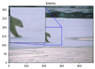
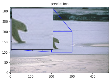
psmr_low: 30.381882136539197 psmr_pre: 29.074438702896636

